- Analysis of the system characteristics regarding observability, controllability, and unforced motion.
Motivation: Before building a controller and an observer, we need to analyze the system whether it is observable, controllable, and its unforced motion. Based on the analysis, we can built the best control system.
-
Equilibrium points
We can find the equilibrium points satisfying the below equation.

The equilibrium points are
 , where
  is any real number
-
Study of observability
Observability can be calculated by  matrix


If 

rank( ) = 3
) = 3
if  , or
, or  rand(4,1)

rank( ) = 4
) = 4
if u is not zero, and 

rank( ) = 4
) = 4
-
Study of controllability

If 

Rank = 3,
if  , or
, or  rand(4,1)

Rank = 4,
- Unforced motion
Simulation result is attached on the next page.
Discussion: First, I found the equilibrium points satisfying the equation, $f=0$, and found the obsevability matrix and controllability matrix at the equilibrium points. The result shows that the system is not observable and not controllable at the equilibrium point. Except the equilibrium the system is observable and controllable. One interesting point is that the system can be observable even at the equilibrium points with control input. This is a unique characteristic which we cannot find in the linear system. Simulation result shows that once the system start from the equilibrium points, the system is completely stable. If the initial state is different with the equilibrium points, x1 (stator current), and x2 (rotor current) converged into the equilibrium points, and once x1 and x2 converged, then x3 (angular velocity) becomes also stable. Because x4 indicates the angular position it becomes larger or smaller continuously.
- Normal form, reduced order manifold (ROM), and zero dynamics.
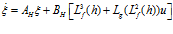
Motivation: Because the system does not have a typical controllability canonical form, I need to transform the system equation into a “normal form” to use a feedback-linearization technique. Feedback linearization is performed when the control input is discovered while differentiating  . If the control input is discovered at the
  -th order differentiation,
  dimensions are not controllable by the feedback linearization technique. Therefore, the dynamics of the remaining part, zero dynamics, should be validated whether it is stable or not.
 ,
, 

 ,
, 


If  ,
,  , stable.
Discussion: The system has the three relative orders, and one remaining order. x2 is not controllable state, and fortunately it converges into zero.
-
Full-state feedback controller.


 is any real number
 matrix


 ) = 3
) = 3 , or
, or  rand(4,1)
 ) = 4
) = 4

 ) = 4
) = 4


 , or
, or  rand(4,1)
 . If the control input is discovered at the
  -th order differentiation,
  dimensions are not controllable by the feedback linearization technique. Therefore, the dynamics of the remaining part, zero dynamics, should be validated whether it is stable or not.
 ,
, 

 ,
, 


 ,
,  , stable.


 is any real number
 matrix


 ) = 3
) = 3 , or
, or  rand(4,1)
 ) = 4
) = 4

 ) = 4
) = 4


 , or
, or  rand(4,1)
 . If the control input is discovered at the
  -th order differentiation,
  dimensions are not controllable by the feedback linearization technique. Therefore, the dynamics of the remaining part, zero dynamics, should be validated whether it is stable or not.
 ,
, 
 ,
, 


 ,
,  , stable.